Deriving the Equation of Motion of a Serial Elastic Actuator
This note shows how I derive the Equation of Motion (EoM) for a 1-dimensional Serial Elastic Actuator (SEA). The main goal is not about the EoM, but rather how can one use a computer algebra system (CAS) to derive equation of motion very easily.
A SEA is a kind of actuator–robot joint–that has a relatively soft spring attached to it, with the goal of reducing impact between the motor with the environment. It allows the engineer to use very high gain in the motor’s controller, and thus allows high precision when needed. It is interesting to note that there are two applications in robotics that SEA are indispensable, but are often known under a different name: the Remote Compliance Center in robotic assembly and the spring-at-the-ankle in humanoids.
The 1D Serial Elastic Actuator model
Let us consider a position-controlled motor attached to a spring-mass as is shown in the hand-drawn figure below.
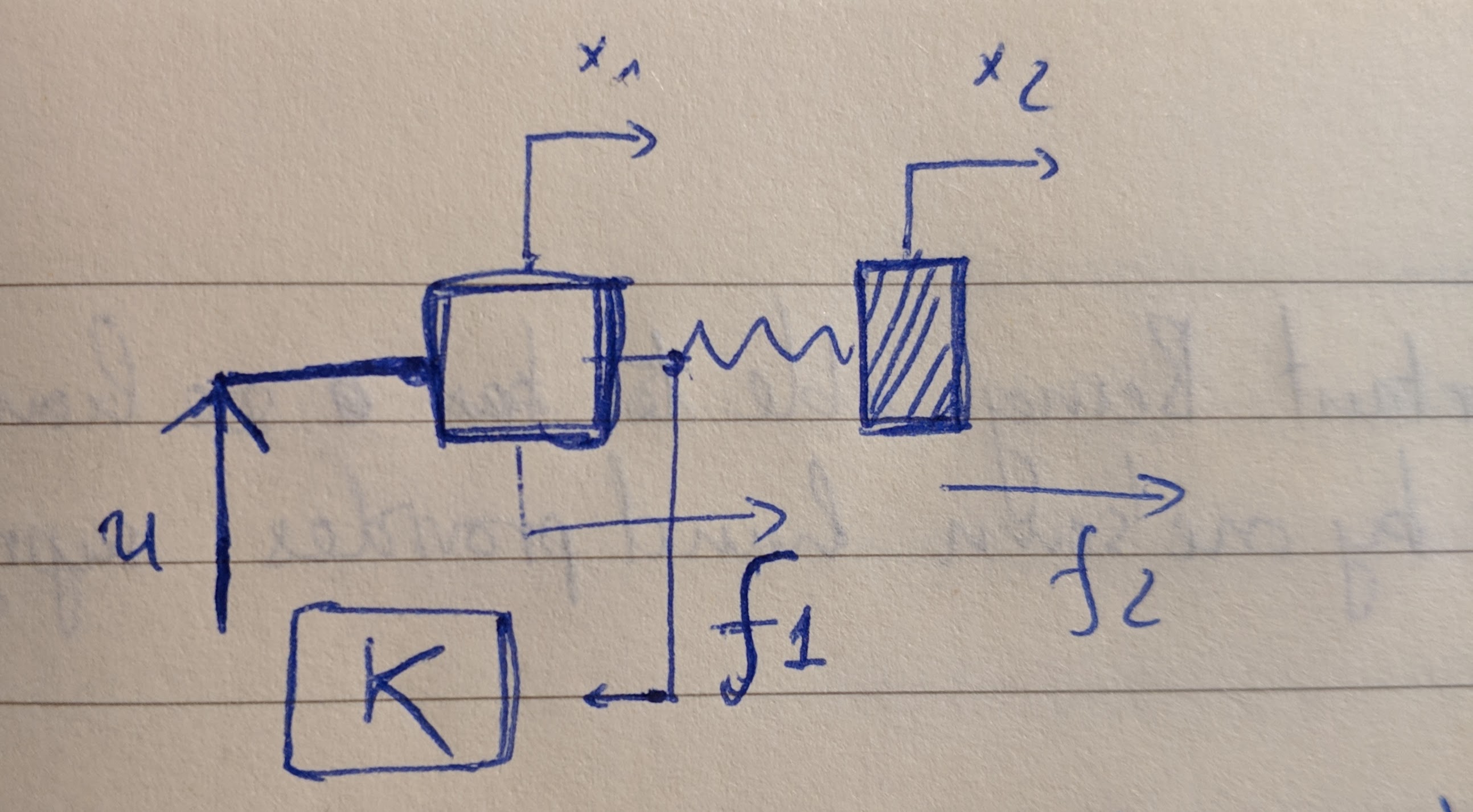
The symbols are respectively:
- \(f_1\): force exerted on the motor by the spring;
- \(f_2\): external force exerted on the mass;
- \(x_1, x_2\): position of the motor and the mass;
- \(u\): position command Additionally, we will use \(k\) for the stiffness of the spring, \(m\) for the mass and \(v_1, v_2\) for the velocities of the motor and the mass.
Suppose now that \(u\) and \(f_2\) are “driving forces” that affect the whole systems, our task in the next part is to derive the equations relating how other quantities are affected by these two driving forces. In fact, we will focus on \(v_2\) and \(f_1\) and call them the outputs of the whole system.
Deriving the Equation of Motion
Two central equations are the force balance equations:
\[f_1 = k( x_2 - x_1), \quad m \ddot x_2 = f_2 + k(x_1 - x_2)\]There are two kinematic equations relating the velocities and positions
\[v_1 = \dot x_1, \quad v_2 = \dot x_2\]And finally, some equation that govern how \(x_1\) is affected by \(u\).
Using the technique invented by Laplace–the Laplace transform–we can turn all the differential equations into algebraic ones. In particular, there are 5 equations. These are:
\[f_1 = k(x_2 - x_1), m x_2 s^2 = f_2 + k (x_1 - x_2)\]and
\[v_1 = x_1 s, v_2 = x_2 s, x_1 = R(s) u\]Note that there are 7 dynamics symbols: \(f_1, f_2, x_1, x_2, v_1, v_2, u\). Therefore, we can solve for all symbols from any two givens ones. This can be done using sympy as follows:
import sympy as sym
Eq = sym.Eq

# dynamic symbols
f1, f2, x1, x2, v1, v2, u = sym.symbols('f1, f2, x1, x2, v1, v2, u')

# "constants"
s, m, b, k = sym.symbols('s, m, b, k ')

R = sym.symbols('R(s)')

equations = [
    Eq(f1, k * (x2 - x1)),
    Eq(m * x2 * s**2, f2 + k * (x1 - x2)),
    Eq(x1, k * u),
    Eq(v1, s * x1),
    Eq(v2, s * x2),
]

sols = sym.solve(equations, [f1, x1, x2, v1, v2])

sols[v2] = sym.expand(sols[v2])
sols[v1] = sym.expand(sols[f1])
The dictionary sols contain the expression for all symbols, except
the inputs $v_2, u$. The output of interest, \(v_2, f_1\) are then
given by: